2026-04-21 — Strobo 2.0 Kickoff

Status: executed 2026-04-21. Parameter-plan record of the main sweep; outcomes are in the companion log 2026-04-21-sweep-complete.md. Author/operator: uwarring (with Claude)

v0.2 edits (2026-04-21, post-preflight). §1 observable list, §4.2, §4.3, §4.4, §5 grid count, §8 execution plan and §9 open questions updated after preflight invalidated the original single-run |C| identity (see §4.2 for details) and to reflect the as-implemented data format (one combined .npz + manifest) and observable count (five reported observables, not three). The original v0.1 text is preserved in git history.

1. Purpose

Map the joint dependence of five observables on two control axes for two short AC pulse-train configurations:

Observables (all defined precisely in §4)
Coherence contrast |C| = √(a_x² + a_y²) — amplitude of the σ_z fringe when scanning the train's analysis phase φ, matching the Hasse Fig. 2(b) "0.76(3)" contrast metric. Extracted from two runs per grid cell (initial spin |+x⟩ and |+y⟩).
Analysis phase arg C = atan2(a_y, a_x) — the value of φ that maximises σ_z.
Spin polarisation ⟨σ_z⟩ at the canonical analysis phase φ = 0 (i.e., sz_A from Run A).
Back-action δ⟨n⟩_A at φ = 0 (Hasse 2024 App. D / Fig. 6b).
Back-action δ⟨n⟩_B at φ = π/2 (companion analysis phase).
Axes
Train detuning δ₀ relative to the atomic carrier, δ₀/(2π) ∈ [−10, +10] MHz.
Initial motional-state phase ϑ₀ ∈ [0, 2π).
Parameterised by
Coherent displacement amplitude |α| ∈ {1, 3, 4.5}.
Train configuration: T1 = (N = 3, δt = 100 ns) and T2 = (N = 7, δt = 50 ns).

Total: 5 observables × 3 α-values × 2 trains = 30 heatmap panels, published as 5 figures of 2 × 3 panels each.

2. Physical parameters (v0.3, 2026-04-21 — π/2-calibrated)

Device-scale parameters (train-independent):

Symbol	Value	Meaning
ω_m/(2π)	1.306 MHz	Motional (LF) frequency
T_m	0.7657 µs	Motional period = 2π/ω_m
η	0.395	Effective Lamb–Dicke parameter
e⁻η²⁄²	0.9250	Debye–Waller factor
Δt	0.770 µs	Inter-pulse spacing
Δt / T_m	1.0056 (+0.56 %)	Slightly super-stroboscopic

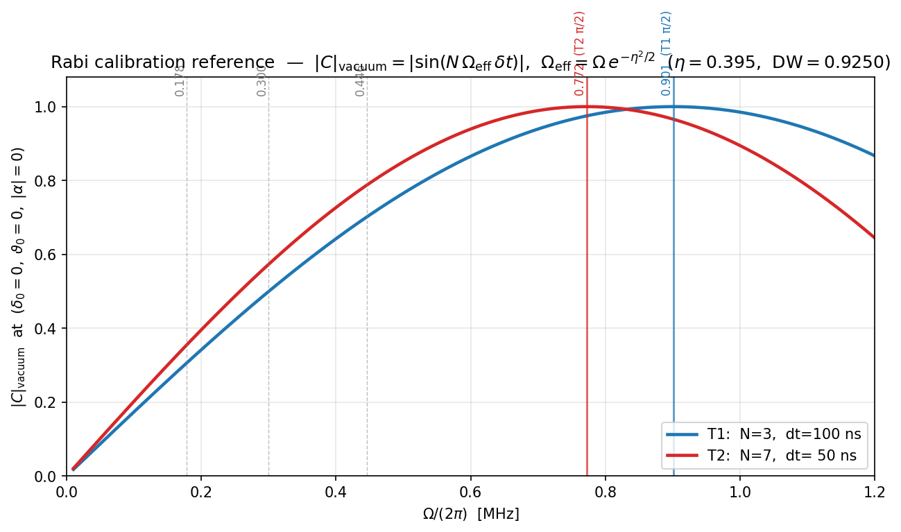
Train configurations, with Ω chosen per train so that N·Ω·e⁻η²⁄²·δt = π/2 (full π/2 analysis rotation on ground motion, matching the Hasse 2024 App. D convention):

Train	N	δt (ns)	Ω/(2π) (MHz)	θ_pulse = Ω·δt·e⁻η²⁄² (rad)	N·θ_pulse (rad)	Total duration
T1	3	100	0.9008	0.5236 (30.0°)	1.5708 = π/2	2·Δt + 3·δt = 1.84 µs
T2	7	50	0.7722	0.2244 (12.86°)	1.5708 = π/2	6·Δt + 7·δt = 4.97 µs

Per-pulse rotation is moderate for T1 (0.52 rad ≈ π/6) and weak for T2 (0.22 rad ≈ π/14). The trains share the same accumulated rotation but distribute it very differently in time. Ω_eff/ω_m ≈ 0.64 (T1) / 0.55 (T2) — both well into the strong-drive regime where a plain Magnus expansion misses important structure; the engine handles this exactly via Fock-basis matrix exponentiation.

Near-stroboscopic-resonant caveat. Δt is 0.56 % longer than T_m. Over a 7-pulse train this accumulates to Δφ_strobo = 2π·7·0.0056 ≈ 14.1° of motional-phase slip from first to last pulse — not negligible for T2. For T1 (2 inter-pulse intervals) the slip is ≈ 4.0°. Flagged for interpretation.

History note. The initial v0.1 run used a single pre-calibration value Ω/(2π) = 0.178 MHz, delivering only N·θ_pulse ≈ π/9 per train (weak probe; max |C| ≈ 0.35). That dataset is superseded by the π/2-calibrated sweep of this v0.3 configuration. The Rabi-rate reconciliation memo is updated accordingly.

3. Sequence layout

  t = 0:   prepare |+x⟩ ⊗ |α e^{i ϑ₀}⟩
  then:    AC pulse train (N pulses, duration δt, spacing Δt, detuning δ₀)
  readout: ⟨σ_x⟩, ⟨σ_y⟩, ⟨σ_z⟩, ⟨n⟩

Initial spin: |+x⟩ = (|↓⟩ + |↑⟩)/√2 for Run A; |+y⟩ for Run B. Experimental equivalent: a perfectly-synchronised MW π/2 that we absorb into state prep.
Initial motion: coherent state |α e^{i ϑ₀}⟩ produced by D(α) with α = |α| e^{i ϑ₀} (convention anchored to the engine; see §6).
Analysis phase φ: the engine's ac_phase_deg is fixed at 0 for all simulations. The experimental φ-scan is recovered by the two-run extraction in §4.2 (init |+x⟩ → a_x; init |+y⟩ → a_y), not by a single-run Bloch-magnitude readout.
Each train is calibrated to a full π/2 analysis rotation on the ground motional state, matching the Hasse 2024 App. D convention. Because T1 (3 × 100 ns) and T2 (7 × 50 ns) differ in N·δt, the required Rabi rate is train-specific:

Ω_T{k}/(2π) = 1 / (4 · N_k · δt_k · e^{−η²/2})

giving Ω_T1/(2π) = 0.9008 MHz and Ω_T2/(2π) = 0.7722 MHz (see §2). This supersedes the single-Ω sweep of the initial strobo 2.0 run, which used the pre-calibration value Ω/(2π) = 0.178 MHz and delivered only N·θ_pulse ≈ π/9. The σ_z(φ) = a_I + a_x cos φ + a_y sin φ fringe structure in §4.2 is kinematic and holds at any N·θ; at the π/2 calibration the fringe amplitude saturates at ≈ 1 on ground motion and the numerical value of |C| becomes directly comparable to the Hasse 2024 "0.76(3)" contrast at |α| ≈ 3. - No separate closing π/2. The train is the only spin-coupling element between state prep and readout — the train is the analysis π/2.

4. Observable definitions

4.1 Back-action (Hasse 2024 definition)

δ⟨n⟩(δ₀, ϑ₀; |α|, N, δt) = ⟨n⟩_fin − ⟨n⟩_ini

with ⟨n⟩_ini = |α|² exactly (coherent initial state) and ⟨n⟩_fin computed from the reduced motional density matrix after tracing out spin. Matches Hasse 2024 App. D and Fig. 6b. The full definition (canonical analysis phase, reporting choice, and units) is in §4.4.

4.2 Coherence and the φ-scan (Protocol-A, Hasse-style)

In Hasse 2024 the AC pulse train is calibrated to a full π/2 analysis rotation (30 × 100 ns), and scanning the train's global phase φ produces a near-unity Ramsey-like fringe. Strobo 2.0 applies the same calibration rule to its shorter trains (§3): each of T1 and T2 is tuned in Ω so that N·Ω·e⁻η²⁄²·δt = π/2. By the lab-frame equivalence U(φ) = R_z(φ) U(0) R_z(φ)†, scanning the train's global phase φ is equivalent to scanning the initial-spin azimuth by −φ, so

⟨σ_z⟩(φ) = a_I(δ₀, ϑ₀) + a_x(δ₀, ϑ₀) cos φ + a_y(δ₀, ϑ₀) sin φ.

The coherence contrast (directly comparable to the "0.76(3)" in Hasse Fig. 2(b), since both are measured under a π/2-calibrated train) is the fringe amplitude:

|C|(δ₀, ϑ₀)   ≡ √(a_x² + a_y²),
arg C(δ₀, ϑ₀) ≡ atan2(a_y, a_x)      (the φ value that maximises σ_z).

On the ground motional state at δ₀ = 0 this saturates at sin(π/2) = 1; finite |α| and finite-δ₀ departures from saturation then produce the structure mapped by this WP.

Preflight 2026-04-21 disproved the single-run identification |C| = |⟨σ_x⟩ + i⟨σ_y⟩| that appeared in the kickoff v0.1 draft. That identity holds only for a Ramsey scheme with a separate closing π/2 at phase φ; the AC-train-as-π/2 protocol of this WP requires two runs per grid cell to isolate a_x and a_y. Preflight measured, at (|α| = 3, δ₀ = 0, ϑ₀ = 0, T2):

⟨σ_x⟩+i⟨σ_y⟩ at φ_laser = 0, init |+x⟩ → magnitude 0.956
Fringe amplitude √(a_x² + a_y²) from 8-point φ-scan → 0.352

These differ by a factor of ~2.7 — the first is the spin Bloch x-y projection after the train, the second is the Hasse coherence. We adopt the second.

Two-run evaluation per (δ₀, ϑ₀) cell.

Run A: spin in |+x⟩ (theta_deg = 90, phi_spin_deg = 0), engine ac_phase_deg = 0. Record sz_A, nbar_A.
Run B: spin in |+y⟩ (theta_deg = 90, phi_spin_deg = 90), engine ac_phase_deg = 0. Record sz_B, nbar_B.

Then (assuming a_I ≈ 0, to be checked):

a_x ≈ sz_A, a_y ≈ sz_B.
|C| = √(sz_A² + sz_B²).
arg C = atan2(sz_B, sz_A).

a_I offset check. At the anchor and at one α = 4.5 point, also run init |−x⟩ (phi_spin_deg = 180) and form a_I = (sz_A + sz(−x))/2, a_x_corr = (sz_A − sz(−x))/2. Proceed with two-run evaluation only if |a_I| ≤ 1 × 10⁻² throughout. If the offset is larger anywhere, promote to a four-run-per-cell evaluation (spins at {+x, +y, −x, −y}).

4.3 σ_z report

σ_z is reported at fixed φ = 0, i.e. sz_A from Run A (initial spin |+x⟩, engine ac_phase = 0). This is the direct read-out at the canonical analysis-phase choice; the arg C heatmap of §4.2 records the phase at which σ_z is instead maximised.

4.4 Back-action report

δ⟨n⟩ is reported at the canonical analysis phase φ = 0 and at its orthogonal companion φ = π/2:

δ⟨n⟩_A (δ₀, ϑ₀) = nbar_A − |α|²   (at φ = 0,   from Run A)
δ⟨n⟩_B (δ₀, ϑ₀) = nbar_B − |α|²   (at φ = π/2, from Run B)

Hasse Fig. 6b shows δ⟨n⟩ over the two-axis (φ, ϑ₀) plane; our sheets are two orthogonal cuts through the analogous surface.

Units. δ⟨n⟩ is reported in raw quanta in the dataset and plot labels; the fractional form δ⟨n⟩/|α|² (Hasse-style, ±1 range) can be recovered by element-wise division at read time, since |α| is recorded in the manifest per sheet. This supersedes the kickoff-v0.1 plan (§9 Q4) of auto-normalising to fractional — keeping the raw numbers in the archive avoids numerical blow-up as |α| → 0 and keeps the reported amplitude directly comparable to the engine's nbar output.

5. Scan grid (confirmed)

Axis	Range	Points
δ₀/(2π)	[−10, +10] MHz, uniform	81
ϑ₀	[0, 2π), uniform	64
	α
Train	{T1 = 3×100 ns, T2 = 7×50 ns}	2

Grid cells: 81 · 64 · 3 · 2 = 31 104 cells. Engine calls: 2 · 31 104 / 81 = 768 calls to run_single, each sweeping 81 detunings internally (2 initial-spin runs × 64 ϑ₀ × 3 α × 2 trains). Fock cutoff: N_max = 60 (ample for |α| = 4.5 with ⟨n⟩ = 20.25; see §8 step 2).

Two distinct reference points are used:

Cross-check anchor: (δ₀ = 0, ϑ₀ = 0, |α| = 0). Reduces to a pure carrier-driven train on the ground motional state; independent check against an analytic LD-expansion prediction (§8 step 1).
Convergence anchor: (δ₀ = 0, ϑ₀ = 0, |α| = 4.5), i.e. the highest-⟨n⟩ cell in the grid. N_max sensitivity is evaluated here as the worst case (§8 step 2).

6. Conventions (engine anchor)

Following scripts/stroboscopic_sweep.py (the intended execution engine):

Motional state: α = |α| · exp(i · ϑ₀) in D(α) = exp(α a† − α* a).
Position quadrature: X = a + a†. → ϑ₀ = 0 prepares the ion on +X̂ (⟨X̂⟩ > 0, ⟨P̂⟩ = 0); ϑ₀ = π/2 prepares on +P̂.
Per-pulse coupling: (ℏΩ/2) · [C(η, a, a†) σ₋ + c.c. σ₊] with C(η, a, a†) = exp(i η (a† + a)), evaluated in the frame rotating at the carrier — detuning δ₀ enters as a free σ_z/2 · δ₀ term during both pulses and inter-pulse intervals.
Inter-pulse free evolution: unitary U_free(Δt) with `H_free = ω_m a†a
(δ₀/2) σ_z` for duration Δt.

7. Expected qualitative features (sanity-check predictions)

Predictions to verify before accepting the sweep data.

δ₀-axis resonances. The ±10 MHz window spans ±7.66 × ω_m, so we expect structure at δ₀ = 0 (carrier) and δ₀ = ±k · ω_m for k = 1, 2, … , 7 (sidebands). Carrier width ≈ Ω_eff/(2π) = 0.178 · exp(−η²/2)/(2π) ≈ 0.165 MHz; individual sideband widths scale as η^k · Ω.
ϑ₀ symmetry. At |α| = 0 the maps are ϑ₀-independent (no displaced state to have a phase). At |α| > 0, periodicity in ϑ₀ is 2π on the σ_z / C observables and π on δ⟨n⟩ (Hasse Fig. 6b shows the characteristic "four-lobe" quadrant pattern at |α| = 3).
Back-action sign. δ⟨n⟩ can be either sign: stroboscopic coupling can cool or heat the motion depending on (δ₀, ϑ₀). Max-|δ⟨n⟩| scales roughly with η · |α| on resonance.
Coherence envelope. |C| is bounded by 1; its maximum on the grid (reached off-resonance at δ₀ ≫ Ω_eff) is ≈ 1. Its minimum at carrier + optimal ϑ₀ is set by N · θ_pulse (≈ 0.34–0.39 rad) and |α|.
T1 vs T2 cross-check. Both trains have near-identical N·θ_pulse (0.335 vs 0.391 rad) but different pulse durations. T2's longer total duration (4.97 vs 1.84 µs) means the ϑ₀ argument drifts more during the train at non-zero detunings; residuals between T1 and T2 at fixed N·θ_pulse isolate this finite-train-duration effect.

8. Execution plan

As executed 2026-04-21 (see 2026-04-21-sweep-complete.md):

Preflight. At the cross-check anchor (δ₀ = 0, ϑ₀ = 0, |α| = 0), verify that the two-run extraction yields real C near the weak-pulse-limit prediction sin(N·θ_pulse). Implemented in numerics/preflight.py.
Convergence check. At the convergence anchor (|α| = 4.5, δ₀ = 0, ϑ₀ = 0), run N_max ∈ {50, 60, 70, 80} and record δ⟨n⟩ convergence. Target: absolute change ≤ 10⁻³ between N_max = 60 and N_max = 80.
φ-scan spot-check. At (|α| = 3, δ₀ = 0, ϑ₀ = 0, T2), run 8 values of φ_laser and fit to a_I + a_x cos φ + a_y sin φ. Confirm max residual ≤ 10⁻¹⁰ and that the two-run extraction (spin {+x, +y}) matches the fit coefficients to ≤ 10⁻³.
Main sweep. 31 104 grid cells over the §5 grid, 768 engine calls total. Save as one combined numerics/strobo2p0_data.npz (keyed by {train}_alpha{|α|}_{observable}) with one numerics/strobo2p0_manifest.json recording parameters, observable contract, and runtime.
Plots. Five figures in plots/, each a 2 × 3 panel array (rows: T1, T2; cols: |α| = 1, 3, 4.5), for a total of 30 heatmap panels covering |C|, arg C, ⟨σ_z⟩, δ⟨n⟩_A, δ⟨n⟩_B.
Logbook. This kickoff, plus follow-up entries (open-ended; one per substantive decision or sub-deliverable). As of 2026-04-21 the WP has four logbook entries total — see the README tree: - this file (parameters, observables, grid); - 2026-04-21-sweep-complete.md (main sweep + qualitative findings); - 2026-04-21-rabi-reconciliation.md (three-candidate Ω read-off protocol); - 2026-04-21-hasse-fig6-slice.md ((φ, ϑ₀) analogue of Hasse Fig. 6 + symmetry checks).

9. Open questions / decisions to confirm

Rabi rate reconciliation. Resolved 2026-04-21 (v0.3): each train is given its own Ω such that N·Ω·e⁻η²⁄²·δt = π/2 (Ω_T1/(2π) = 0.9008 MHz, Ω_T2/(2π) = 0.7722 MHz). Matches the Hasse 2024 App. D convention. See 2026-04-21-rabi-reconciliation.md for the five candidate values considered and plots/00_rabi_calibration.png for the |C|_vacuum curve.
Inclusion of a pre-train MW π/2. Treated as perfectly absorbed into state prep (|+x⟩). Include it explicitly if experimentally the MW π/2 duration is comparable to Δt and its free-evolution contribution to the motional phase matters. Default: absorbed.
Δt = 0.77 µs vs T_m = 0.7657 µs. Deliberate choice or round value? If deliberate, this WP reports the "near-stroboscopic-slip" regime; if round, a second run at Δt = T_m exactly would isolate the slip effect.
δ⟨n⟩ normalisation for publication. Resolved in §4.4: archive stores raw quanta; fractional form is a read-time derivation. The plots in this WP also display raw quanta; a Hasse-style fractional comparison figure can be generated in a follow-up pass if needed.
Noise model. Pure-state unitary for this WP. If experimental comparison becomes a goal, add decoherence per WP-E §4a D2 protocol.

10. Provenance

Engine: extension of scripts/stroboscopic_sweep.py (Float64, exact Fock-basis matrix exponentiation via scipy.linalg.expm).
Reference paper: Hasse, Palani, Thomm, Warring, Schaetz, Phys. Rev. A 109, 053105 (2024) — App. C (Hamiltonian) and App. D (back-action definition + Fig. 6 qualitative comparison).
Sibling WPs: wp-phase-contrast-maps/ — N = 22 weak pulses, δt = 40 ns, phase-contrast forward map.

v0.1 2026-04-21 — initial draft. v0.2 2026-04-21 — observable contract corrected after preflight. v0.3 2026-04-21 — per-train π/2 calibration: Ω is train-specific, §2 rewritten accordingly, §3 sequence layout reframed as "π/2 analysis pulse per train," §4.2 caveat removed (|C| is now directly comparable to Hasse 2024 Fig. 2(b)), §9 Q1 resolved.